IEEE Visualization 2004 Contest Entry
PDF: PDF Document
Video: Video
Slides: PowerPoint
OpenGL Visualization of Hurricane Isabel
Authors
- Greg P. Johnson, Texas Advanced Computing Center, gregj@tacc.utexas.edu
- Christopher A. Burns, Texas Advanced Computing Center, cslugg@tacc.utexas.edu
Contest Entry Visualization System
Our visualization solution is an OpenGL application we designed and developed specifically to visualize this data set. The code is written in C/C++ and uses the GLUT toolkit for user input and frame buffering. We have also made use of the FLTK library for GUI controls, and an implementation of the Pthreads API for multithreading. We chose this strategy so that we would best be able to customize the visualization features to suit this particular data set, and to maximize the interactivity of the visualization. Multithreading is used to effectively perform I/O and sorting operations in parallel, while GUI controls give the user an easy way to set various parameters related to visual quality, performance, and the transfer functions used to represent data.
Criterion 1: Interactivity
Real-time performance of our solution was a design goal from the beginning. Our program by default will downsample the precipitation data by a factor of four in each dimension, the wind data by a factor of ten in the X and Y dimensions, and the cloud data is left at full resolution. However, the user can dynamically downsample the data further to improve performance if necessary. Our hardware consists of a Dell system with two Intel Xeon processors running at 2.8 GHz, 2.0 GB of memory, and an NVIDIA GeForce 6800 GT graphics card. There are three different sets of variables which can be enabled or disabled by the user: clouds, wind, and precipitation. At a resolution of 800x600 and with all three sets enabled, we can achieve a frame rate of approximately 13 fps. When the clouds are disabled, frame rate improves to 30 fps. While the simulation is running and new data is constantly being streamed from disk and interpolated, these values drop to 5 fps and 13 fps respectively.
Criterion 2: Exploratory Support
The user is able to manipulate the camera view easily during any mode or phase of the simulation (while paused, or while the simulation plays through the timesteps). The movement of the camera is quite standard and therefore is easy to use. The mouse controls the look direction and the arrow keys on the keyboard control movement through space. The camera can be trucked along the view direction, from side to side, or along the camera's "up" axis. These features are sufficient to allow the user to closely examine any part of the visualization at any time during the simulation.
While the simulation automatically advances the visualization along the timeline by default, the user may pause at any time, or instruct the program to jump to any particular timestep. The data is interpolated between the given timesteps to ensure smooth transitions between them for intermediate frames. Thus the user has full flexibility to scan through the time-varying data automatically, or can inspect any particular timestep statically.
Criterion 3: Multiple Characteristics
Clouds and Structure
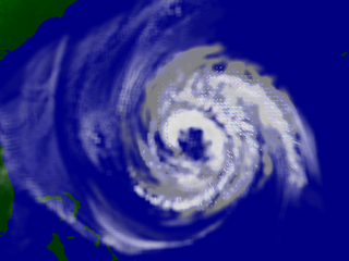
To display the clouds we used a particle system where each cloud particle is rendered with a single billboarded quad. The saturation and transparency of the particles are linear functions of the cloud data and are set by default such that heavy clouds result in darker and more opaque particles, resulting in a cloud that looks thick. As the camera travels through the rendered particles, the clouds appear to thin out, just as real clouds do. Sorting of the partially transparent quads is achieved by subdividing the volume into a series of 3D tiles which are sorted by their centroids' distance from the camera. The particles in each tile are then sorted in parallel. The tiling allows us to reduce the computational complexity of sorting the cloud particles, and since the arrangement of the data in memory reflects the tiling, our program achieves a more coherent memory access pattern which makes better use of the processors' cache memories.
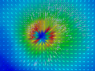
Wind Velocity
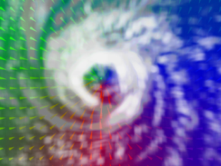
The wind data can optionally be visualized simultaneously with the cloud and precipition data. Using a horizontal slicing plane, the wind values are illustrated with a grid of colored vectors and a partially transparent surface. The colors can be computed by mapping the color wheel onto the compass directions, with red indicating north. Alternatively, the colormap can relate wind magnitude, with warmer colors indicating stronger winds. The vectors' length is a linear function of the wind magnitude at that voxel. The altitude of this plane and vector field can be adjusted by the user at any time.
Precipitation
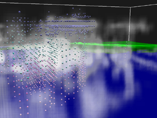
The precipitation variables are rendered using a simple particle technique that makes it easy to visualize the precipitation along with the cloud structure in the same frame. For a given voxel, the precipitation is represented by a colored sphere. Cyan spheres indicate graupel, magenta corresponds to rain, blue indicates snow, and gray represents the total precipitation. The saturation of a particle is determined by a linear transfer function of the variable's ratio data value, and the function's parameters are user configurable. The discrete particles show up well against the background of the cloud structures, which are rendered in a way that looks more volumetric. It is important that the users be able to effectively visualize the cloud structure and the precipitation simultaneously.
Additional Comments
The sheer size of the data set presented the biggest obstacle to our goal of producing an interactive visualization that is both aestetically pleasing and scientifically informative. We expended considerable effort optimizing the memory layout, reducing the frequency of I/O operations, and eliminating unnecessary geometric processing on the GPU. While our solution is not necessarily complete (due to subsampling), we compensate for this by allowing the user to adjust the degree to which certain variables are subsampled as appropriate. Finally, we have not implemented any visualization of the temperature, pressure, or ice mixing ratio variables due to time constraints. However, the methods used to visualize other similar variables could easily be extended to illustrate these. Other improvements to our solution might include more user control over the transfer functions, slicing planes along other axes, and more precise control over the camera.